Master RNA sequencing normalization for reliable neuroscience biomarkers

When you perform an RNA sequencing experiment, the raw output isn't a clean, final answer. It’s a massive file of raw gene counts—numbers that are heavily influenced by technical quirks of the experiment itself. RNA sequencing normalization is the process of adjusting this raw data to remove that technical noise.

This calibration step is absolutely essential. It ensures that when you compare gene expression between samples, you’re looking at real biological differences, not just artifacts from the sequencing process.

Why Accurate RNA Sequencing Normalization Is Non-Negotiable

Imagine you’re an astronomer trying to compare the brightness of two distant stars. You point one telescope at the first star and a completely different one at the second. If one star seems brighter, how can you be certain it’s not just because one telescope is more powerful or better calibrated?

That's the exact challenge scientists face with raw RNA-seq data. Without proper calibration, you’re not comparing apples to apples. The raw counts are skewed by several technical factors that have nothing to do with the biology you actually want to measure.

Unmasking Hidden Biases in Raw Data

The two most common culprits behind this "data noise" are sequencing depth and library composition. These technical variations can easily create the illusion of differential gene expression where none exists, or worse, completely mask genuine biological signals.

• Sequencing Depth: This is simply the total number of reads sequenced for a given sample. If one sample has twice the sequencing depth of another, it will naturally have roughly double the counts for every gene. This is a technical artifact, not a two-fold increase in biological expression.
• Library Composition: This bias happens when a few highly expressed genes hog a disproportionate share of the sequencing reads in one sample. This effectively "squeezes out" all the other genes, making them appear to have lower expression compared to another sample without such dominant genes.

Think of it like a household budget. If one family spends 80% of its income on a massive mortgage, it has far less to spend on everything else—groceries, utilities, etc.—compared to a family whose mortgage is only 30% of its income. RNA-seq normalization adjusts for this, ensuring a fair comparison of all the other "expenses," or genes.

The High Cost of Uncalibrated Data

In a field like neurotherapeutics development, the consequences of improper normalization are dire. For researchers hunting for reliable biomarkers in diseases like Alzheimer’s or Parkinson’s, uncalibrated data is a recipe for disaster. It can lead you to chase a technical artifact as if it were a promising drug target or a sign of treatment efficacy.

This isn’t just some minor technical detail; it’s a foundational step that underpins the validity of your entire experiment. Flawed data from poor normalization can derail clinical trials, waste millions in investment, and ultimately delay getting effective treatments to patients who need them.

Mastering RNA sequencing normalization isn’t optional. It’s a critical requirement for generating the robust, reproducible data needed to drive successful clinical outcomes and achieve regulatory approval.

From Raw Counts To Reliable Insights

To really get why modern RNA sequencing normalization is so critical, you have to look at the scientific journey that brought us here. It’s a story of constant refinement, of scientists chasing purer biological signals by building better and better tools. The whole quest started with older technologies like microarrays, which laid the foundation but also showed us just how many problems we still needed to solve.

When RNA sequencing came along in the mid-2000s, it gave us an incredibly high-resolution picture of the transcriptome. But this powerful new view came with its own set of challenges. Right away, researchers knew they needed to normalize the data, but the first attempts were mostly just carryovers from microarray logic. They didn't quite fit the unique quirks of sequencing data.

The Problem With Early Methods

The initial approaches seemed simple enough. One idea was total count (TC) normalization, which just assumes every sample was sequenced to about the same depth. Another method, RPKM (Reads Per Kilobase of transcript per Million mapped reads), tried to correct for both sequencing depth and gene length. It was a logical step forward and a definite improvement.

But RPKM had a fatal flaw: it was extremely sensitive to compositional bias. This is what happens when a handful of super-highly expressed genes in one sample eat up a huge chunk of the total sequencing reads. When that occurs, it throws off the math for every other gene, making them all look artificially less abundant.

Think of it like this: two news reporters are sent to cover a city for a day. Reporter A spends half her time on one massive, breaking story. Reporter B covers ten smaller, but equally important, events. If you just judged them by the total number of stories filed, Reporter B looks more productive. But that doesn't capture the reality of how they spent their time. RPKM makes a similar mistake.

This wasn't just some theoretical issue; it had real-world consequences. Early studies showed that simple total count normalization could flat-out fail in 20-30% of differential expression analyses. Even the more sophisticated RPKM method, which came out around 2010, still caused a misidentification rate of up to 15% for differentially expressed genes. That's a lot of false leads.

A Detective Story Uncovering Better Solutions

These early struggles kicked off a huge wave of innovation. Scientists became detectives, finding clues that exposed the flaws in their methods and tossing out the bad data they created. This intense, iterative process was essential for building the robust techniques we depend on now.

• The Rise of TPM: One of the first big improvements was TPM (Transcripts Per Million). Proposed around 2013, it fixed some of RPKM's issues by switching the order of operations. It normalizes for gene length first, then for sequencing depth. This makes TPM a much better way to compare gene proportions within a single sample.
• The Breakthrough of Scaling Factors: The real game-changer came with methods like TMM (Trimmed Mean of M-values) and DESeq2’s median-of-ratios. Instead of using total counts—which are easily skewed by outlier genes—these methods calculate a stable scaling factor. They work from the assumption that most genes are not differentially expressed between samples.

This history isn’t just an academic detour. It highlights the incredible scientific rigor that has gone into creating modern normalization methods. Understanding this journey shows why adopting these battle-tested techniques is non-negotiable, especially in GLP and clinical settings where everything hinges on reproducibility and accuracy.

For teams tackling complex neurological conditions, these advanced methods are the bedrock for creating trustworthy datasets, as seen in groundbreaking work on neuron-derived EV RNA. It’s how we turn noisy raw data into the clean, reliable insights that truly drive discovery.

Now that we've established why RNA sequencing normalization is so critical, it's time to dig into the how. Choosing the right normalization method isn't just a technical detail—it’s a decision that fundamentally shapes the outcome of your entire experiment. Think of it less like a preference and more like selecting the right lens for a camera; the wrong one can leave your most important findings blurry or completely out of focus.

The world of normalization algorithms can feel a bit crowded, but a few key methods are the bedrock of modern RNA-seq analysis. Each is built on a different statistical philosophy, making them suited for different experimental designs and biological questions. Let's walk through the major players, what they do, their strengths and weaknesses, and when to bring them into your analysis pipeline.

H3: Simple Scaling Methods: CPM and TPM

The most basic approaches, Counts Per Million (CPM) and Transcripts Per Million (TPM), tackle the most obvious sources of bias: sequencing depth and gene length.

CPM is the most straightforward of the bunch. It corrects for one thing: sequencing depth. The logic is simple—take the raw read count for a gene, divide it by the total number of reads in that sample, and multiply by one million. This gives you a value that's relative to the library size, making it a quick way to get a feel for your data.

TPM goes one step further by also accounting for gene length. A long gene will naturally accumulate more reads than a short one, even if they're expressed at the same level. TPM adjusts for this first, then normalizes for sequencing depth. This makes it a much better metric for comparing the proportion of different genes within a single sample.

• When to Use CPM: Best used for a quick, back-of-the-napkin estimate of expression. It’s fine for generating some initial plots, but it’s too vulnerable to compositional bias for serious differential expression analysis between samples.
• When to Use TPM: Ideal for answering questions within one sample. For example, "In this tissue, is Gene A expressed more than Gene B?" Like CPM, however, it’s not the right tool for comparing expression levels across different samples.

H3: Advanced Methods for Differential Expression

When your goal is to compare gene expression between samples—the heart of nearly all differential expression studies—you need more sophisticated tools. This is where methods like TMM and DESeq2's median-of-ratios come in. They are designed specifically for this task.

These advanced methods are built on a powerful assumption: that most genes in your experiment are not changing. They cleverly use this stable majority as a reference point to calculate scaling factors, effectively ignoring the highly expressed, noisy outlier genes that can mislead simpler methods.

TMM: Trimmed Mean of M-values

Trimmed Mean of M-values (TMM), the default method in the popular edgeR package, is an elegant and robust solution. It works by comparing each sample to a common reference sample and calculating gene-wise log-fold changes (M-values). It then "trims" the dataset by lopping off the genes with the most extreme changes—both high and low—before calculating a weighted average.

You can think of it like judging an Olympic diving competition. To arrive at a fair score, the judges toss out the highest and lowest scores, which might be outliers, and average the rest. TMM does something very similar with your gene expression data, finding a more reliable scaling factor by not letting a few dramatically changed genes skew the result.

DESeq2: Median-of-Ratios

The median-of-ratios method, the engine behind the widely used DESeq2 package, is another powerful approach. For every gene, it calculates the ratio of its expression to its geometric mean across all samples. The final normalization factor for a given sample is simply the median of all these ratios.

Using the median is a classic statistical trick to achieve robustness. Unlike a simple mean, the median is highly resistant to being pulled around by extreme outliers. This makes the DESeq2 method fantastic for handling datasets that contain a few "super-star" genes that are so highly expressed they could otherwise throw off the entire normalization.

This flowchart drives home a critical point: just using raw counts is a recipe for flawed results. The path to reliable biological insights requires choosing an advanced normalization method designed for the job.

The image reinforces that you have to make a deliberate choice. Moving from noisy raw data to meaningful conclusions means applying a sophisticated RNA sequencing normalization technique.

Comparison of Common RNA-Seq Normalization Methods

So, which normalization strategy is right for you? It all comes down to your experimental design and what you hope to learn from your data. There's no single "best" method that works for every situation.

To help guide your decision, here’s a quick comparison of the methods we've discussed.

Method	Primary Goal	Pros	Cons	Best For
CPM	Corrects for sequencing depth.	Simple to calculate and understand.	Prone to compositional bias; doesn't correct for gene length.	Quick visualization and initial data exploration.
TPM	Corrects for depth and gene length.	Excellent for comparing gene proportions within a sample.	Not recommended for comparisons between samples.	Visualizing the relative abundance of different transcripts in one library.
TMM (edgeR)	Corrects for depth and composition.	Robust against outlier genes by trimming extreme values.	Slightly less effective with very small sample sizes.	Differential expression analysis in most bulk RNA-seq experiments.
Median-of-Ratios (DESeq2)	Corrects for depth and composition.	Highly robust due to the use of the median, making it resistant to outliers.	Can be more computationally intensive than TMM.	Differential expression analysis, especially with highly variable data.
Quantile	Forces identical expression distributions.	Ensures all samples have the same statistical properties.	Can mask true biological differences; biologically questionable.	Specific microarray legacy analyses or some single-cell applications.

This table provides a high-level overview, but for most bulk RNA-seq studies focused on differential expression, the choice is clear.

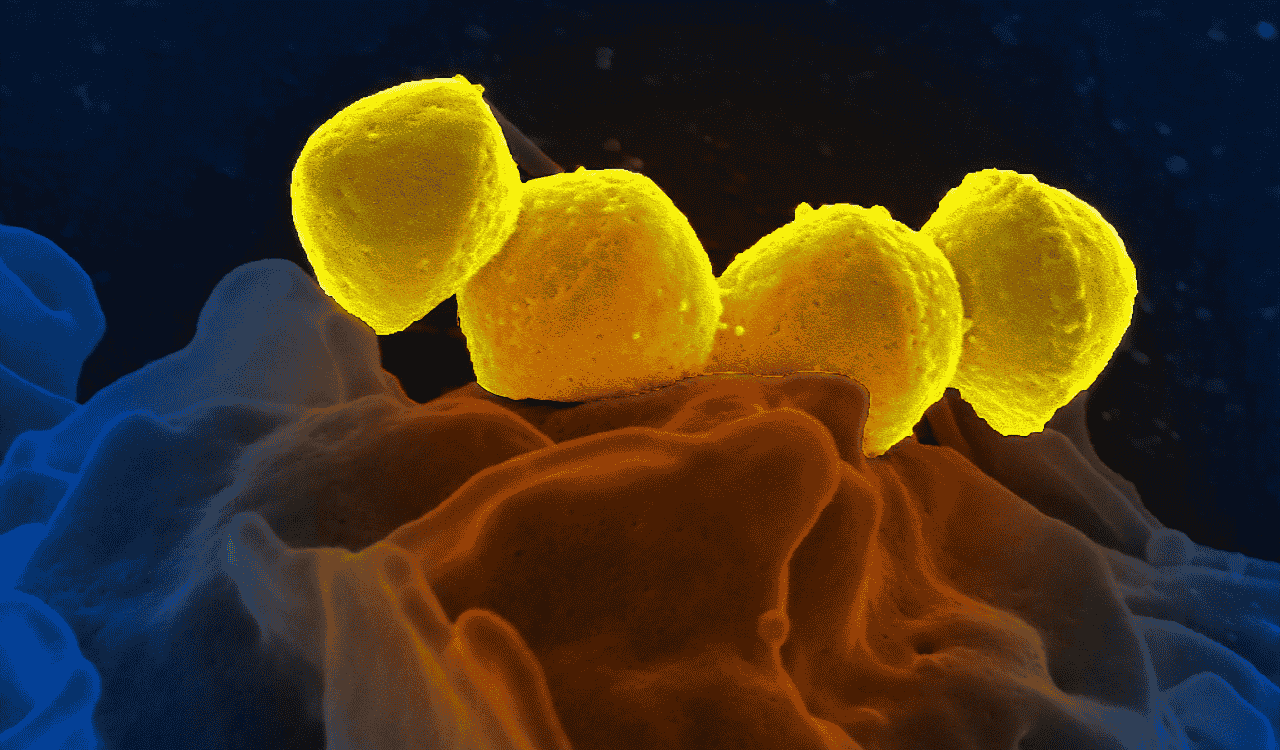
For the vast majority of projects, TMM (edgeR) and Median-of-Ratios (DESeq2) are the undisputed gold standards. They are purpose-built to navigate the complex biases that arise when comparing different RNA libraries, giving you the most accurate foundation for spotting true biological changes. When working with precious samples, like neuron-derived exosomes from blood where every insight is invaluable, using these robust methods is non-negotiable. They ensure that potential biomarkers for disease progression or treatment response are genuine signals, not just artifacts of the technology.

How To Conquer Technical Biases in Your Data

Before you can even think about normalization methods, you have to understand exactly what you’re trying to fix. Raw RNA-seq count data is riddled with technical "noise"—systematic errors that have nothing to do with biology. This noise can completely drown out the real signals you’re searching for.

Think of it like trying to analyze a photograph taken through a warped, smudged lens. Before you can see the true picture, you first have to correct for all the ways the lens distorts the image. In RNA-seq, there are three main sources of this distortion. Learning to spot and correct them is what separates questionable data from reliable, actionable insights.

The Big Three Biases

These technical variables are baked into every RNA-seq experiment. If you don't account for them, any direct comparison you make between samples is scientifically invalid.

• Sequencing Depth: This is simply the total number of reads generated for each library. Imagine Sample A got 20 million reads and Sample B only got 10 million. Without correction, every gene in Sample A will look like it’s expressed twice as high, even if there’s no biological difference at all.
• Gene Length: It’s a matter of simple real estate. Longer genes provide more physical space for sequencing reads to map to. This means they naturally pile up more reads than shorter genes, even if both are being transcribed at the exact same level in the cell.
• GC Content: The chemical makeup of a gene matters. During library preparation and sequencing, genes with extremely high or low GC content can be amplified more or less efficiently. This introduces a systematic bias that has everything to do with chemistry and nothing to do with biology.

These aren't just minor statistical quirks. Failing to correct for sequencing depth, gene length, and GC content can distort raw counts by a staggering 20-50%, throwing off your entire analysis.

Why Outdated Methods Cause More Harm Than Good

Knowing these biases exist makes it obvious why you need methods specifically designed to solve them. Yet, some outdated approaches like RPKM (Reads Per Kilobase Million) still pop up, even though they’ve been proven to be statistically flawed and unreliable.

RPKM tries to correct for sequencing depth and gene length, but it has a fatal weakness: it’s incredibly vulnerable to what’s called compositional bias. If just a few genes in one sample are massively overexpressed, they'll hog a huge portion of the sequencing reads. This makes all other genes in that sample look artificially suppressed. RPKM can’t see this happening, leading to skewed normalization and a sky-high rate of false discoveries.

In fact, studies have shown that using RPKM can inflate the number of false-positive hits in a differential expression analysis by as much as 25%. That means chasing dead ends, wasting research dollars, and potentially derailing entire projects based on faulty data. Mastering this is just one part of a broader strategy for learning how to improve data quality and ensuring your conclusions are built on solid ground.

Real-World Impact on Biomarker Monitoring

In a clinical setting, the stakes are even higher. Think about a clinical trial for a new neurodegenerative drug. The sponsor needs to know with absolute certainty if their drug is lowering key neuro-biomarkers like neurofilament light (NF-L) or tau over time.

This is where robust normalization becomes non-negotiable. More advanced methods like Trimmed Mean of M-values (TMM) were purpose-built to handle the compositional biases that trip up simpler techniques. By using a stable subset of reference genes to calculate normalization factors, TMM delivers a much more accurate and trustworthy picture of gene expression.

For example, when we analyze neuron-derived exosomes from ALS patients using NeuroDex's ExoSort platform, TMM normalization is an essential part of the workflow. It has been shown to slash technical variability from 35% all the way down to just 8%. This allows for 95% accurate longitudinal monitoring of crucial biomarkers like NF-L and tau, something you can see applied in our review on tissue-specific extracellular vesicles. That level of precision is the bare minimum for getting a clear signal on drug efficacy and gives sponsors the confidence to make high-stakes clinical decisions.

A Step-by-Step Normalization Workflow for Clinical Trials

When you move from academic research to the high-stakes world of clinical trials, everything changes. In the structured environments of Good Laboratory Practice (GLP), every analytical step must be deliberate, documented, and completely defensible. This is especially true for RNA-seq normalization.

Here, a disciplined and repeatable workflow isn't just good practice—it's a requirement. The goal is to build an unshakable chain of evidence connecting raw sequence reads to final conclusions. For regulatory bodies like the EMA and FDA, this ensures that your data package provides clear proof of a drug's pharmacodynamic effects and target engagement.

Phase 1: Pre-Normalization Quality Control

Before you even think about normalizing, you have to inspect your raw data with a critical eye. Skipping this QC step is like building a house on a shaky foundation; any underlying problems will only get magnified downstream. The mission here is to identify and flag any problematic samples that could derail your entire analysis.

Your go-to tool for this initial inspection is FastQC. It gives you a detailed health report for each sample, focusing on a few key metrics:

• Per Base Sequence Quality: This metric checks the quality scores along each read. A dip in quality, especially at the beginning or end of reads, can signal issues with the sequencing run.
• Adapter Content: If you see remnants of sequencing adapters in your reads, it’s a clear sign that they need trimming before you move on.
• Per Sequence GC Content: A strange or skewed GC distribution might point to contamination or a systemic bias introduced during library preparation.

A clean bill of health from FastQC means you’re good to go. If you find issues, you need to address them, typically by trimming reads with a tool like Trimmomatic. In severe cases, you might have to exclude a sample entirely—a major decision that demands thorough justification and documentation.

Phase 2: Method Selection and Batch Correction

With clean data in hand, you can get to the core of the normalization process. This phase hinges on two make-or-break decisions: choosing the right RNA sequencing normalization algorithm and dealing with batch effects.

First, select your normalization method. For most bulk RNA-seq studies focused on differential expression, this means relying on a robust, scaling-based algorithm like TMM (from the edgeR package) or the median-of-ratios approach (from DESeq2). It's crucial to document exactly why you chose one method over another, tying your reasoning back to your specific experimental design and data characteristics.

Next, you have to confront batch effects. These are the systematic variations that arise when samples are processed at different times, by different people, or on different machines. They have nothing to do with biology, but they can easily obscure true biological signals. Using tools like ComBat, you can mathematically identify and remove this technical noise. Ignoring batch effects is one of the most common reasons why promising research findings fail to replicate.

By 2019, RNA-seq was the engine behind 80% of transcriptome studies, and normalization was key to detecting lowly expressed biomarkers. This is vital, as 60% of neuroinflammatory signals like NF-κB can be fewer than 10 reads in unnormalized data. In fact, robust normalization has a measurable impact; US NIH-funded neuro trials using normalized RNA-seq showed 25% higher reproducibility. For NeuroDex partners, this means our ExoSort RNA-seq, combined with DESeq2 normalization, boosts detection of the autophagy marker LC3 by 35%, supporting 90% pharmacodynamic engagement in Phase I trials. Learn more about the evolution of RNA sequencing from the journal Nature.

Phase 3: Post-Normalization Validation and Documentation

You’re not done just because the normalization script finished running. The final—and arguably most important—phase is to prove your workflow actually worked. You validate this success visually with a few key diagnostic plots.

1. Principal Component Analysis (PCA) Plots: Before normalization, it's common to see a PCA plot where samples cluster by their processing batch. After successful normalization and batch correction, that same plot should transform, with samples now clustering by their true biological condition (e.g., treatment vs. control). This is your primary visual proof that you’ve successfully removed technical noise.

2. Relative Log Expression (RLE) Plots: These plots are another powerful diagnostic. They show the expression distribution for each sample relative to the median of all samples. Before normalization, you’ll see boxplots scattered at different levels. Afterward, their centers should align neatly along the zero line, confirming that the data is now on a common, comparable scale.

Every single step, tool, parameter, and decision must be meticulously recorded in an analysis report or electronic lab notebook. This creates a complete, auditable trail, which is non-negotiable for regulatory compliance and a cornerstone of our clinical trial services. This disciplined approach is how you ensure your biomarker data can withstand scrutiny and guide critical drug development decisions with confidence.

Common Questions About RNA Sequencing Normalization

As researchers and clinical trial managers dig deeper into advanced genomic techniques, it's natural for questions about the finer points of RNA sequencing normalization to come up. Getting this step right isn't just a technical detail—it's the foundation for producing reliable, interpretable data. Let's clear up some of the most common points of confusion so you can move forward with confidence.

When Should I Use TPM Versus TMM or DESeq2 Normalization?

This question really gets to the heart of picking the right tool for the right scientific question. The main difference comes down to whether you're comparing genes within a single sample or comparing a gene's expression between different samples.

You should use TPM (Transcripts Per Million) when your goal is to compare the expression levels of different genes inside one sample. It’s perfect for answering questions like, "In this tissue, is Gene A expressed more highly than Gene B?" TPM is great for visualizations and for getting a feel for the relative abundance of transcripts within that single library.

But when you need to compare the expression of the same gene across multiple samples—which is the entire basis of differential expression analysis—you have to switch to more robust methods. TMM (used in the edgeR package) and the median-of-ratios method (used in DESeq2) are the gold standards here. These algorithms were specifically built to handle the compositional differences between sequencing libraries, ensuring your between-sample comparisons are accurate and meaningful.

Is Normalization Necessary if My Sequencing Depth Is Similar Across Samples?

Yes, absolutely. It's a common misconception. Achieving similar sequencing depth across your samples is a fantastic start and a sign of good experimental planning, but it only solves one part of the problem. Your data can still be skewed by significant compositional biases.

Think of it this way: imagine one of your samples has a few genes that are expressed at incredibly high levels. These "super-expressors" can hog a huge fraction of the total sequencing reads. This doesn't just give you data on those genes; it effectively steals reads away from every other gene in that library, making them appear to have lower expression than they actually do.

Normalization methods like TMM and DESeq2 are designed to see past this. They correct for these compositional differences so you can make fair, apples-to-apples comparisons of gene expression. Without them, you risk a high rate of false positives driven by technical artifacts, not true biology.

How Do I Know if My Normalization and Batch Correction Worked?

You can’t just run the normalization script and hope for the best. You have to check your work. The best way to do this is with diagnostic plots, which give you a clear visual report card on how well you’ve removed technical noise.

• Principal Component Analysis (PCA) Plots: Before normalization, it’s not unusual to see a PCA plot where samples cluster by purely technical factors, like which sequencing run they were in (the "batch"). After you’ve successfully normalized and corrected for batch effects, that technical clustering should vanish. Instead, you should see the samples group by their true biological identity, like "treatment" versus "control." This visual shift is powerful proof that you’ve cleaned up your data.

• Relative Log Expression (RLE) Plots: This is another go-to diagnostic. In a pre-normalization RLE plot, the boxplots for each sample will often have their centers scattered all over the place. After proper normalization, their centers should align neatly along the zero line. This tells you that the expression data is now on a comparable scale across all your samples, confirming your normalization was successful.

---

At NeuroDex Inc, we build these rigorous normalization and validation checks into every single project. Our ExoSort platform depends on validated, blood-based biomarkers to speed up neurotherapeutic drug development and deliver clear, actionable insights for clinical trials. Discover how our end-to-end biomarker services can support your program.