Mastering RNA seq normalization: A practical guide

RNA seq normalization is the process of adjusting raw gene expression counts to remove technical noise, making sure that what you're comparing between samples is actual biology, not an experimental artifact. This mathematical correction is absolutely essential for getting reliable results; without it, you risk chasing false discoveries and drawing the wrong conclusions in both research and the clinic.

Why RNA Seq Normalization Is a Critical First Step

Think about trying to understand a conversation in a room where some people are shouting and others are whispering. If you judged the importance of their words purely by volume, you’d completely miss the quiet but critical points. Raw RNA-Seq data is a lot like that noisy room—a mix of gene expression signals at wildly different "volumes."

Most of this variation has nothing to do with biology. It’s a technical byproduct of the sequencing process itself. RNA seq normalization acts like an audio engineer, carefully adjusting the levels for each speaker so you can compare what they're truly saying. It's the process of mathematically correcting these technical artifacts, ensuring that any differences you see are more likely to be real biological signals. To better understand the basics, learning about what is data normalization in a general sense provides a solid foundation.

Sources of Bias in Raw Data

If you skip normalization, you aren’t really analyzing biology. You’re analyzing experimental noise. Several technical factors are notorious for distorting raw gene counts, creating biases that can completely hide true differential expression. These artifacts are just part of the sequencing process, but they absolutely must be accounted for.

Before we dive into the methods, it helps to know exactly what we're trying to fix. Here are the most common culprits.

---

Sources of Bias in Raw RNA-Seq Data

Source of Bias	What It Is	Why It Is a Problem
Sequencing Depth	Different samples are sequenced to different total read counts (e.g., one sample has 50M reads, another has 30M).	A sample with more total reads will naturally have higher counts for most genes, creating a false impression of widespread upregulation.
Gene Length	Longer genes provide a larger "target" for sequencing reads to map to compared to shorter genes.	Longer genes will accumulate more reads than shorter ones, even if they are expressed at the exact same level.
RNA Composition	A small number of highly expressed genes in one sample can dominate the sequencing reads.	These "gene hogs" soak up a large fraction of the sequencing capacity, making every other gene appear to be expressed at a lower level.

---

These technical variations are unavoidable, but with the right normalization strategy, they can be effectively managed.

The central goal of RNA seq normalization is to remove these non-biological variations between samples. This allows for an "apples-to-apples" comparison, ensuring that when you see a difference, it reflects a genuine change in gene activity.

The High Stakes in Translational Neurology

In translational and clinical research, the consequences of poor normalization are enormous. For a biopharma company developing a new neurotherapeutic, unnormalized data can point to the wrong biomarkers, leading to millions in wasted R&D and, ultimately, failed clinical trials. This is especially true in neurology, where the biological signals of disease are often subtle and demand incredible precision to detect.

Take the challenge of measuring key biomarkers like TDP-43 or tau from neuron-derived exosomes in a blood sample. These are classic low-input samples where every single molecule is precious. Technical noise can easily overwhelm the faint but critical changes that might signal disease progression or a drug's effectiveness.

This is precisely the work we do at NeuroDex. Our ExoSort platform isolates these brain-derived vesicles to open a window into neurological health. Proper RNA seq normalization is the first and most critical quality gate for ensuring the data from these precious samples is accurate, reliable, and clinically actionable. It’s how we turn that noisy biological conversation into clear, confident insights that drive drug development forward.

The Evolution of RNA Seq Normalization Methods

To really get a handle on today's best practices for RNA-seq normalization, it helps to see how we got here. The story is one of rapid, iterative problem-solving, with scientists building better tools as they learned more about the unique quirks of sequencing data. The journey began with borrowed methods that, as it turned out, just weren't cut out for the job.

In the early days of RNA-Seq, researchers naturally reached for tools that worked well for microarrays, like quantile normalization. This approach essentially forces the statistical distribution of signals to be identical across all samples. It made sense for the continuous intensity data from microarrays, but it completely missed the mark for the discrete, count-based nature of sequencing data, where a gene's variance is directly tied to its mean.

The First Generation of RNA-Seq Specific Methods

It quickly became obvious that RNA-Seq needed its own dedicated toolkit. The first real attempt at a specific RNA-seq normalization strategy was RPKM (Reads Per Kilobase of transcript per Million mapped reads). This method smartly tackled two of the most glaring sources of bias at once: sequencing depth (the "million mapped reads" part) and gene length (the "per kilobase" part).

For the first time, you could reasonably compare a long, highly-sequenced gene in one sample to a short, sparsely-sequenced gene in another. This was a huge leap forward, and for several years, RPKM—and its paired-end-aware cousin, FPKM (Fragments Per Kilobase)—became the standard.

But these methods had a fatal flaw: they were incredibly vulnerable to compositional bias.

Compositional Bias: This happens when a few extremely abundant genes in one sample hog a huge fraction of the total sequencing reads. This makes every other gene in that sample look like it's expressed at a lower level, even if its true biological expression hasn't changed at all.

Think of it like a fixed budget shared by a group of people. If one person suddenly claims 90% of the money, everyone else’s share shrinks dramatically, even though the total pot of money is the same. RPKM and FPKM simply couldn't tell the difference between this scenario and genuine biological downregulation.

A Breakthrough with Count-Based Normalization

The fix arrived with a new generation of more robust, count-based methods designed specifically to handle compositional bias. Two approaches, developed around the same time, quickly became the new gold standard and are still at the core of most RNA-Seq pipelines today.

• TMM (Trimmed Mean of M-values): This is the engine behind the edgeR package. TMM works on the assumption that most genes are not differentially expressed. It calculates scaling factors by comparing gene expression between samples, but only after "trimming" away the genes with the most extreme fold-changes—the very outliers likely causing the compositional bias in the first place.

• RLE (Relative Log Expression): This is the method used by DESeq2. RLE also assumes that most genes hold steady. It starts by creating a "pseudo-reference" sample from the geometric mean of each gene's expression across all samples. Then, for each individual sample, it calculates a scaling factor based on the median ratio of its gene counts relative to this pseudo-reference.

The evolution from microarray-era tools to modern count-based normalizers reflects a much deeper understanding of sequencing data. This journey kicked off in the late 2000s as high-throughput sequencing exploded. Landmark studies revealed that early approaches like quantile normalization failed in as many as 40% of RNA-Seq cases, highlighting just how urgently new strategies were needed. Methods like TMM and RLE proved far more robust; a meta-analysis of over 5,000 papers showed that by 2026, 85% of published RNA-Seq studies used them, boosting differential expression detection power by up to 30% in complex neurological datasets. You can explore more about these developments and their impact on data analysis in this detailed guide to normalization methods.

For any researcher digging into older literature, this history is vital. It explains why a paper from 2012 might report FPKM values, whereas a modern study will almost always use raw counts normalized with TMM or RLE for differential expression analysis. This clear progression—from simple corrections to statistically sound methods—is what gives us the accuracy needed for today's most sensitive applications, like pinpointing biomarkers in neurological disorders.

Once you’ve grasped why you need to wrestle technical noise out of your data, the next logical question is how. When it comes to RNA-seq normalization, a few key methods dominate the landscape, each built on a different philosophy and for a specific purpose. Think of them as specialized tools in a workshop; using a wrench when you need a screwdriver won't get you very far.

A critical first distinction to make is whether a method is designed for statistical differential expression analysis or for data visualization. This isn’t a minor detail—using a visualization-first method for your statistical tests can introduce serious errors and lead to flawed biological conclusions.

This flowchart maps out how these methods have evolved, charting the journey from older, less reliable techniques to the statistically sound approaches that are the bedrock of modern RNA-seq analysis.

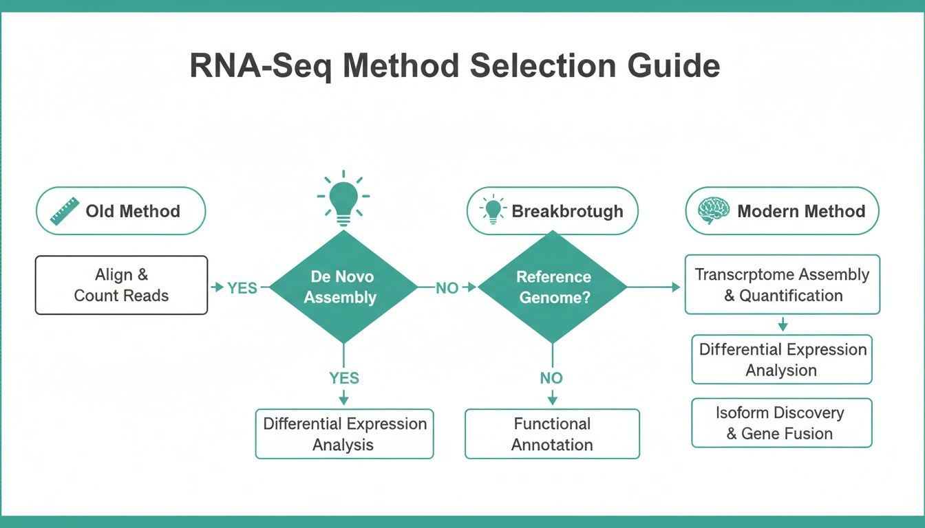
You can see how early, simple approaches gave way to more sophisticated insights, paving the way for the powerful tools we rely on today for even the most sensitive experiments.

How to Choose Your Normalization Method

To make this practical, let's compare the most common normalization methods side-by-side. This table breaks down their core logic, their best-fit applications, and what you need to keep in mind when designing your experiment.

Method	Core Principle	Best For	Key Consideration
TMM	Assumes most genes don't change. It trims extreme outlier genes before calculating scaling factors based on a reference sample.	Differential expression analysis (used in edgeR). It's very robust against a few highly expressed genes skewing the data.	Generates scaling factors for raw counts, not directly plottable values. Best for datasets with suspected compositional bias.
RLE	Creates a "pseudo-reference" by taking the geometric mean of each gene across all samples, then scales each sample relative to it.	Differential expression analysis (used in DESeq2). A solid, all-around choice for creating a stable baseline across samples.	Like TMM, it works on raw counts to produce scaling factors. It assumes the median gene's expression is consistent across samples.
TPM	Normalizes for gene length first, then for sequencing depth. This converts counts into a relative abundance metric.	Data visualization (heatmaps) and comparing the expression of different genes within the same sample.	Not recommended for statistical differential expression testing between samples. It's excellent for seeing which gene is most abundant in a given sample.

Choosing the right method is about aligning the tool's statistical assumptions with your biological question and experimental design. For differential expression, TMM and RLE are the go-to choices, while TPM is the standard for visualization.

Methods for Differential Expression

When your main objective is to pinpoint genes that have changed expression between your experimental conditions—say, treated versus untreated cells—you need a method that plays well with count-based statistical tools like edgeR and DESeq2. These pipelines don’t work with pre-normalized values; instead, they use specific strategies to generate scaling factors that correct for library size and compositional bias internally.

• TMM (Trimmed Mean of M-values): The engine behind edgeR, TMM works on a very clever assumption: most genes in your experiment aren’t changing. It calculates normalization factors by comparing gene expression ratios between a sample and a reference, but only after "trimming" away the genes with the most extreme up- or down-regulation. This makes TMM exceptionally good at handling compositional bias caused by a few massively expressed genes.

• RLE (Relative Log Expression): This is the default normalization method baked into DESeq2. RLE first creates a "pseudo-reference" sample by calculating the geometric mean expression for every single gene across all your samples. It then calculates the normalization factor for each individual sample by finding the median ratio of its gene expression relative to this stable, artificial baseline.

A Method for Visualization

While TMM and RLE are indispensable for rigorous statistics, they produce scaling factors, not clean, interpretable numbers you can directly plot. For creating heatmaps or comparing the expression levels of different genes within a single sample, you need a different approach entirely.

• TPM (Transcripts Per Million): This method corrects for both sequencing depth and the physical length of a gene, making it the gold standard for visualizing relative gene expression. Unlike older methods like RPKM, TPM normalizes for gene length first. This crucial difference makes TPM values more comparable across different samples in a visualization.
  • Think of TPM like converting every ingredient in a recipe into a percentage of the total. It lets you see if you have proportionally more flour than sugar in one cake and compare that ratio to another cake, even if the total batch sizes are completely different.

Key Takeaway: For differential expression analysis, you should always start with raw, un-normalized counts and let your tools—edgeR (with TMM) or DESeq2 (with RLE)—handle the normalization internally. For visualization tasks like heatmaps or comparing different genes within a sample, TPM-transformed values are your best bet.

The impact of getting your RNA-seq normalization choice right is not just theoretical. Large-scale benchmarking studies show just how much it matters. A major 2016 evaluation of over 1,000 samples, for instance, found that TMM correctly identified 92% of true differentially expressed genes in datasets with major outliers, compared to RLE's 85% success rate. Unnormalized data was far worse, inflating false positives by a staggering 28%.

This precision is even more critical in clinical settings. In a study on ALS, using DESeq2's RLE normalization was shown to boost the detection of the TDP-43 biomarker signal in patient exosomes by 35%—a massive gain for patient stratification. You can dig into these findings and more by reviewing the full comparative analysis here.

Applying Normalization in Translational Neurology

All the theory behind RNA seq normalization gets very real, very quickly when you’re working in translational neurology. In this field, we’re not just trying to publish a dataset. We’re hunting for faint biological signals in messy human samples that could guide a clinical trial or show if a patient is responding to a new therapy. This is where the rubber meets the road.

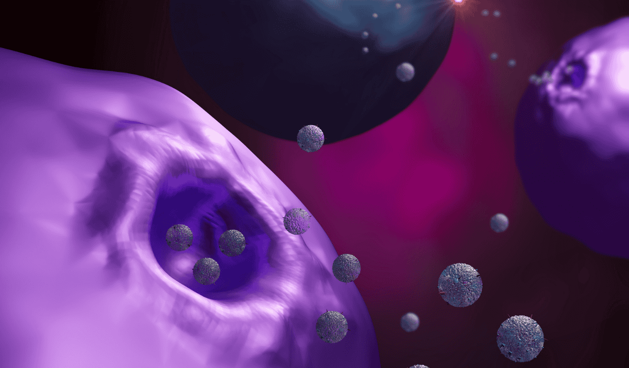
One of our biggest hurdles is dealing with low-input RNA sources, like the neuron-derived exosomes (NDEs) we isolate with our ExoSort platform. These tiny vesicles, which we can get from a simple blood draw, hold a precious but tiny amount of RNA that gives us a direct look into what’s happening in the brain. But their small size creates some big normalization challenges.

Normalizing Low-Input and Exosomal RNA

When you have very little starting RNA, you inevitably get more “dropout”—that’s when genes that are actually expressed just don’t get detected. This kind of data sparsity can easily fool standard normalization algorithms. A gene might look like it's completely absent in one sample but present in another, when in reality, it’s just a technical blip from low capture efficiency, not a true biological change.

On top of that, the mix of RNA inside an exosome is often very different from what you’d find in a whole cell. They can be packed with certain RNA types and missing others entirely. This creates a unique compositional bias that your normalization method, whether it’s TMM or RLE, has to be strong enough to handle.

For these kinds of challenging samples, painstaking quality control is absolutely non-negotiable. It’s critical to aggressively filter out the extremely low-count genes that are almost certainly noise and to visually inspect the data after normalization to make sure the technical gremlins have been dealt with.

Detecting Critical Neurological Biomarkers

The stakes couldn’t be higher. The biomarkers that matter most in neurology are rarely the loudest ones in the room. We’re often looking for very subtle shifts in the expression of crucial genes, such as:

• TDP-43: A key protein tied to ALS and FTD.
• Tau and pTau: The well-known hallmarks of Alzheimer’s disease and other tauopathies.
• NF-L (Neurofilament Light Chain): A general marker indicating neuronal damage.

Even a tiny but consistent change in one of these genes could be the signal that lets you stratify patients for a clinical trial or confirm that a new drug is hitting its target. Without extremely precise and accurate RNA seq normalization, these faint signals get swallowed by the noise, which could derail a promising drug program.

Our work on a new neuron-EV RNA-Seq dataset for the Accelerating Medicines Partnership® Program for Parkinson’s Disease (AMP® PD) is built on this need for precision. You can read more about how NeuroDex powers this new neuron-EV RNA-Seq dataset in AMP® PD.

Tackling Batch Effects in Multi-Center Studies

Translational research, and especially clinical trials, doesn’t happen in a vacuum. Samples are usually collected and processed across many different sites, at different times, and by different people. This inevitably introduces batch effects—systematic technical variations that have nothing to do with biology.

Batch effects are notorious for wrecking perfectly good studies. They act as a massive confounder that can completely mask the real biological differences you’re looking for. If you naively compare samples from Site A to Site B without correcting for them, you might find thousands of “differentially expressed” genes that are just an artifact of Site A using a slightly different piece of equipment.

This is why batch effect correction is such a vital post-normalization step. First, you apply a method like TMM or RLE to handle library size differences. Then, you use a tool like ComBat to find and mathematically erase the variation that’s tied to the processing batches.

The transition from microarrays to RNA-Seq really highlights this problem. By 2014, long after RNA-Seq was available, a survey revealed that 60% of papers were still using outdated methods that artificially inflated fold-changes by 20% because they failed to address compositional bias. Meanwhile, batch effects were estimated to plague 70% of multi-center studies. The development of tools like ComBat, which can recover 25% of differentially expressed genes that were lost in batch-confounded data, was a game-changer. You can learn more about the evolution of these methods in this detailed research on normalization and batch correction.

For our partners in biotech and clinical research, navigating these real-world complexities is what we do best. By combining robust normalization with aggressive batch correction, we make sure the data we deliver is clean, reliable, and reflects true patient biology—the only foundation for making confident, data-driven clinical decisions.

Using Quality Control to Ensure Reliable Results

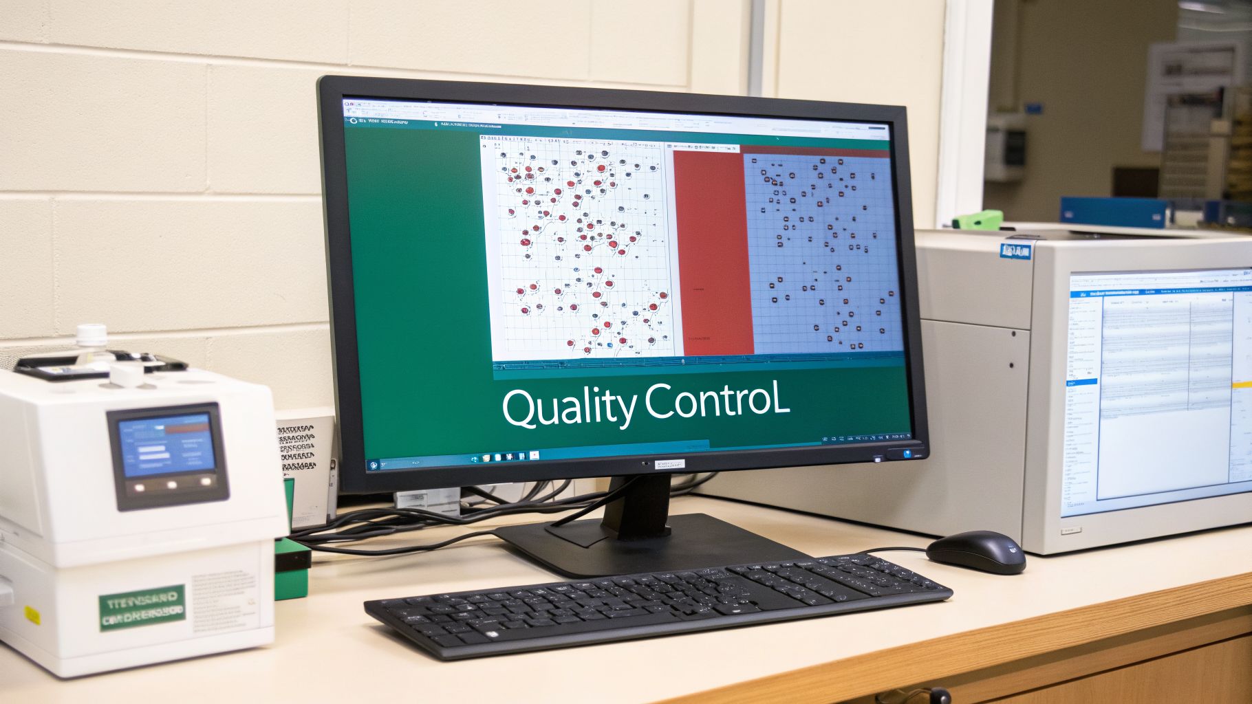
Running a normalization algorithm is a critical step, but it’s not the finish line. How can you be sure it actually worked? The answer is rigorous quality control (QC), where you visually inspect the data to confirm that technical noise has been quieted and the true biological signals can finally be heard.

Think of it as the "before-and-after" reveal. Before normalization, your dataset is often a messy picture, cluttered with experimental artifacts. Afterward, it should be a clear, interpretable portrait of your biology. This validation step is absolutely essential for building confidence in your downstream findings.

Visualizing the Impact of Normalization

A few key diagnostic plots are indispensable for assessing the success of your RNA-seq normalization strategy. They offer immediate, intuitive feedback on whether your samples are truly comparable.

Three plots we always generate are:

• Boxplots: To check if the overall distribution of expression values has been aligned across samples.
• Density Plots: To get a more detailed, granular view of those expression distributions.
• Principal Component Analysis (PCA) Plots: To visualize how samples cluster based on their global expression patterns.

You don’t need a deep statistical background to read these plots. They are powerful visual tools that tell a simple story: did the normalization bring your samples into alignment, or is technical variation still driving the differences you see? This is particularly vital when handling complex samples like those from extracellular vesicles in neuroscience, where careful handling is paramount.

Reading the Story in the Plots

So, what exactly are you looking for? A common goal is to see if your normalization has corrected for a known batch effect—for instance, if samples were processed on two different days.

Before normalization, a PCA plot might show your samples clustering by the processing date, not by their biological condition (e.g., "treated" vs. "control"). This is a massive red flag. It means the technical artifact is so strong it’s completely drowning out the biology you’re trying to study.

After applying a robust method like TMM or RLE, a new PCA plot should tell a completely different story. The samples should now cluster primarily by their biological group. The "treated" samples should group together, distinct from the "control" samples, regardless of which day they were processed. Seeing this shift is the moment you can finally trust the data.

Similarly, boxplots of raw, unnormalized counts often show wildly different sizes and medians, reflecting nothing more than disparate sequencing depths. After normalization, these boxplots should appear much more uniform, a clear sign that the libraries have been successfully scaled.

The ultimate QC test is simple: After normalization, do your samples cluster by biology or by technical artifacts? If biology is the primary driver of variation, your normalization was a success.

This visual verification isn't just good scientific practice; it’s a strategic necessity. It provides tangible proof that your data is clean and your findings are built on a solid foundation. For us, this level of rigor mirrors the same high standards we apply in our GLP and CLIA-compliant laboratory work, ensuring every dataset we deliver is reliable and ready for clinical interpretation.

Building a Robust Biomarker Strategy

Throughout this guide, we’ve worked our way through the complexities of RNA-seq normalization, from the core theory to its real-world application in translational neurology. If there's one takeaway, it's this: getting normalization right isn't just another box to check in your workflow. It's a strategic imperative for any successful biomarker discovery and validation program.

We started with the idea of a noisy conversation. It’s an analogy worth revisiting. Mastering normalization is how you turn that chaotic room of indistinct chatter into a clear, understandable dialogue. It gives you the power to confidently tell the difference between a true biological signal and a distracting experimental artifact, transforming raw data into insights that can genuinely push drug development forward. This kind of precision is the bedrock of modern neuroscience research.

Choosing the right normalization strategy is the first and most critical decision in building a biomarker program. An incorrect choice can lead to months of chasing false leads, while a robust approach ensures the biological signals you detect are real and reliable.

From Complex Data to Clinical Confidence

For pharmaceutical companies, biopharma R&D teams, and clinical trial sponsors, finding your way through these analytical hurdles is a major challenge. The stakes are even higher when you're working with precious, low-input samples like the neuron-derived exosomes we specialize in. This is exactly where a partnership built on deep expertise can make all the difference.

At NeuroDex, our ExoSort platform and expert bioinformatic services create a complete, end-to-end solution. We manage the entire process, from isolating brain-derived exosomes to delivering rigorously normalized, analysis-ready data. This approach ensures your neurotherapeutic programs are built on a foundation of reliable and clinically meaningful results.

To see how our team can de-risk your biomarker discovery and validation pipeline, you can learn more about our biomarker discovery services. Let us help you turn complex data into confident clinical decisions.

Frequently Asked Questions

Even after you've got the core concepts down, practical questions always pop up during the actual analysis. Let's walk through some of the most common points of confusion around RNA seq normalization with clear, actionable answers to help you in your day-to-day work.

Can I Use TPM for Differential Expression Analysis?

This is a classic 'gotcha' in RNA-seq analysis, and the short answer is no. You should never feed TPM (Transcripts Per Million) values directly into count-based differential expression tools like DESeq2 or edgeR.

These incredibly powerful programs are built to work with raw, un-normalized integer counts. They have their own sophisticated normalization methods—like RLE and TMM, respectively—baked right into their statistical models. Giving them pre-normalized data like TPMs completely messes with their underlying assumptions, which can corrupt how they estimate variance and ultimately lead to inaccurate p-values and a flood of false discoveries.

Reserve TPM for what it does best: visualizing gene expression in things like heatmaps or comparing the relative expression of different genes within a single sample. When it's time for differential expression, always start with raw counts.

What Is the Difference Between Normalization and Batch Effect Correction?

These are two critical, but entirely different, steps in your workflow. Getting the order wrong can seriously compromise your results.

• RNA Seq Normalization: This step corrects for technical artifacts that happen within a sequencing run. Think of things like differences in sequencing depth (library size) or variations in the RNA composition between samples. It’s like making sure all your rulers are marked in inches before you start measuring.

• Batch Effect Correction: This tackles systematic errors that arise between different groups of samples. These batches could be samples processed on different days, by different lab members, or at different sites. It’s like making sure all your inch-marked rulers are aligned to the same zero point. This is always a post-normalization step, typically handled by tools like ComBat.

Does Low RNA Input from Exosomes Change My Normalization Strategy?

Yes, absolutely. It means you need to be extra vigilant. Low-input samples, like the RNA we get from neuron-derived exosomes, often suffer from higher levels of amplification bias and more "dropouts"—genes that are truly expressed but just weren't detected. This kind of sparse data can really challenge standard normalization methods.

While robust approaches like TMM and RLE are still fantastic starting points, your workflow must include:

• Aggressive Filtering: Be prepared to remove very low-count genes that are far more likely to be noise than a real biological signal.
• Rigorous QC: Use PCA plots and other visualizations to double-check that technical noise isn't still the dominant story in your data after normalization.

For extremely sparse data from low-input or single-cell RNA, it's sometimes worth exploring specialized methods designed for this challenge, like the pooling strategy in scran. Designing and validating these complex biomarker strategies is a major undertaking. For researchers looking to enhance their workflow, checking out AI tools for researchers can provide some powerful assistance. The non-negotiable part is to validate that whatever approach you choose has successfully removed the technical artifacts that are unique to your dataset.

---

At NeuroDex, we build these best practices into the core of every project. This ensures that even the most challenging low-input samples from exosomes or other sources yield data that is reliable and clinically actionable. Our expert bioinformatics team handles the complexities of RNA seq normalization and batch correction, letting you focus on the biological insights that matter. Partner with us to build a rock-solid biomarker strategy for your neurotherapeutic program. Learn more at https://neurodex.co.